In a previous blog posting I considered that the disparity between the Ipsos Reid and Forum Research results may be due to the methodology in how this polling is done. In this blog I will detail how I arrived at the final result.
When we attempt to find a solution that matches the polling results exactly a solution is possible only if \(p=0\). To include other values of \(p\) we have to relax this notion and instead consider solutions that match as close as possible in some sense. That is, to find \(\vec{\alpha}\) such that some measure of distance between the Ipsos Reid and Forum Research results are minimized. Mathematically we can say that we are looking for\[\vec{\alpha}^* = \underset{\vec{\alpha}}{\operatorname{argmin}}\| \vec{b}_{\textrm{I}}-(p\vec{b}_{\textrm{F}}+(1-p)\vec{\alpha}\|,\]where \(\vec{b}_{\textrm{I}}=(0.36,0.20,0.28,0.13,0.03,0)^\top\) and \(\vec{b}_{\textrm{F}}=(0.31,0.31,0.27,0.16,0.02,0.03)^\top\) are the Ipsos Reid and Forum Research data from the table. The double vertical bars mean that we are taking a norm and there are a number of choices that could be made. For convenience we take the Euclidean norm. Other notions of distance such as the Manhattan norm or the max norm could be used. In a finite dimensional vector space (in our case 6-dimensional for the 6 lines in the table) all these these norms are equivalent but they are typically much more computationally intensive and may require the use of sub-differential algorithms (quantifying change at points of non-differentiability). Finally the notation \(\operatorname{argmin}\) denotes that we want to minimize something and that rather than know what this minimum is, we are interested in extracting where the minimum occurs.
However, there are also a number of constraints. In particular, each of the \(\alpha_i\) is a proportion and taken together, they should give 100%. This translates into the constraints that \(0 \le \alpha_i\le 1 \ \forall i\) and \(\alpha_1+\alpha_2+\alpha_3+\alpha_4+\alpha_5+\alpha_6=1\). Each of these constaints, all 13 of them give a separate condition. Defining \begin{align*}f(\vec{\alpha};p) &= \| \vec{b}_{\textrm{I}}-(p\vec{b}_{\textrm{F}}+(1-p)\vec{\alpha}\|_2^2,\end{align*}and\begin{align*}g_{1,i}(\vec{\alpha}) &= -\alpha_i \le 0,&g_{2,i}(\vec{\alpha}) &= \alpha_i – 1 \le 0,&
h(\vec{\alpha}) &= \sum_{i=1}^6\alpha_i – 1 = 0
\end{align*}allows us to state the problem in a standard form.
For any \(0\le p\le 1\) find \[\vec{\alpha}^* = \underset{\vec{\alpha}}{\operatorname{argmin}}f(\vec{\alpha};p)\] subject to\begin{align*}g_{1,i}(\vec{\alpha})&\le 0, & g_{1,i}(\vec{\alpha})&\le 0, & h(\vec{\alpha})&=0.
\end{align*}This is known as a nonlinear programming problem in the optimization literature and there are a number of algorithms to efficiently solve this problem numerically. In our case the function \(f\) is strictly convex (being a norm), \(g_{i,j}\) is linear and therefore convex and \(h\) is affine. These conditions ensure that for each value of \(p\) there is a unique optimal distribution that can be found.
The necessary condition for optimality are known as the Karush-Kuhn-Tucker (KKT) conditions and they take the following form. If \(\vec{\alpha}\) is a nonsingular optimal solution of our problem, then there exist multipliers \(\mu_{1,i}, \mu_{2,i}, \lambda\) such that \begin{align*}\nabla_{\vec{\alpha}}f(\vec{\alpha};p) + \sum_{i=1}^6\mu_{1,i}\nabla_{\vec{\alpha}}g_{1,i}(\vec{\alpha}) + \sum_{i=1}^6\mu_{2,i}\nabla_{\vec{\alpha}}g_{2,i}(\vec{\alpha}) + \lambda\nabla_{\vec{\alpha}}h(\vec{\alpha})&=0,\\ \textrm{for} \ i = 1,2,\ldots,6: \quad \mu_{1,i}g_{1,i}(\vec{\alpha})=0,\quad \mu_{2,i}g_{2,i}(\vec{\alpha})=0,\\ \textrm{for} \ i = 1,2 \ \textrm{and} \ j = 1,2,\ldots,6: \quad \mu_{i,j}\ge 0, \quad g_{i,j}(\vec{\alpha}) \le 0, \quad h(\vec{\alpha})&=0.\end{align*}The first line is a condition that will pick up any minimum and maximum values, the second line chooses which of the constraints are active and the third line filters out only those that are feasible. One of the roadblocks to a solution is the number of possible combinations of constraints that can be chosen. In this case there are \(2^{12} = 4096\) possibilities, although this can be reduced by using the structure of the problem. For example, if one of the \(\alpha_i = 1\) then all the other \(\alpha_i\) must be zero. A naive method would be to try all 4096 possibilities and then patch them together as \(p\) increases from 0 to 1.
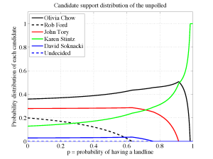
Rather than sacrificing myself on this alter of 4096 possibilities, I first attempted to find a solution where \(0 < \alpha_i < 1\) (no equalities) so that \(\mu_{1,i}=\mu_{2,i}=0 \forall i\) but as was found earlier, this solution is only feasible if \(p=0\). What it also revealed is that for small positive \(p\), it was \(\alpha_6\) that became negative so I moved to the constraint \(\mu_{1,6}=0\) to force \(\alpha_6=0\) and deflate the problem to finding the remaining 5 \(\alpha_i\) values. This yields the partial solution \begin{align*}\vec{\alpha}(p) &= \frac{1}{1-p}\begin{pmatrix}0.36-0.316p\\0.20-0.316p\\0.28-0.276p\\0.13-0.066p\\0.03-0.026p\\0\end{pmatrix}, & 0\le p&\le \frac{0.20}{0.316}\simeq 0.6329,\end{align*} with \(\alpha_2=0\) being the terminating condition. This behaviour implied that the next patch should result from setting \(\mu_{1,2}=\mu_{1,6}=0\) to force \(\alpha_2=\alpha_6=0\) and continue the deflation process. Continuing,\begin{align*}\vec{\alpha}(p) &= \frac{1}{1-p}\begin{pmatrix}0.41-0.395p\\0\\0.33-0.355p\\0.18-0.145p\\0.08-0.105p\\0\end{pmatrix}, & 0.6329\le p&\le \frac{0.08}{0.105}\simeq 0.7619,\end{align*} with \(\alpha_5=0\) defining the upper extent of the domain,\begin{align*}\vec{\alpha}(p) &= \frac{1}{3(1-p)}\begin{pmatrix}1.31-1.29p\\0\\1.07-1.77p\\0.62-0.54p\\0\\0\end{pmatrix}, & 0.7619\le p&\le \frac{1.07}{1.17}\simeq 0.9145,\end{align*} with \(\alpha_3=0\) at the upper limit, \begin{align*}\vec{\alpha}(p) &= \frac{1}{1-p}\begin{pmatrix}0.615-0.625p\\0\\0\\0.385-0.375p\\0\\0\end{pmatrix}, & 0.9145\le p&\le \frac{0.615}{0.625}= 0.984,\end{align*} terminated by \(\alpha_1 \to 0\) and finally\begin{align*}\vec{\alpha}(p) &= \begin{pmatrix}0\\0\\0\\1\\0\\0\end{pmatrix}, & 0.984\le p&\le 1.\end{align*}
Concatenating all these cases together results in the figure displayed below. This mathematical technique is commonly used in inverse problem concerning deblurring, tomography and super-resolution. Essentially we can think of this as taking an x-ray of the total voting public and not just those that appear on the surface through their landline.